Model

Given a classification problem, one of the more straightforward models is the logistic regression. But, instead of simply presenting it and using it right away, I am going to build up to it. The rationale behind this approach is twofold: First, it will make clear why this algorithm is called logistic regression if it is used for classification; second, you’ll get a clear understanding of what a logit is.

Well, since it is called logistic regression, I would say that linear regression is a good starting point. What would a linear regression model with two features look like?

A linear regression model with two features

There is one obvious problem with the model above: Our labels (y) are discrete; that is, they are either zero or one; no other value is allowed. We need to change the model slightly to adapt it to our purposes.

What if we assign the positive outputs to one and the negative outputs to zero?

Makes sense, right? We’re already calling them positive and negative classes anyway; why not put their names to good use? Our model would look like this:

Logits

\(\color{red}{\text{Equation above Mapping a linear regression model to discrete labels.}}\) To make our lives easier, let’s give the right-hand side of the equation above a name: logit (z).

Computing logits

The equation above is strikingly similar to the original linear regression model, but we’re calling the resulting value z, or logit, instead of y, or label.

Does it mean a **logit is the same as linear regression?**

Not quite—there is one fundamental difference between them: There is no error term (epsilon) in Equation above. If there is no error term, where does the uncertainty come from? I am glad you asked :smiley: That’s the role of the probability: Instead of assigning a data point to a discrete label (zero or one), we’ll compute the probability of a data point’s belonging to the positive class.

Probabilities

If a data point has a logit that equals zero, it is exactly at the decision boundary since it is neither positive nor negative. For the sake of completeness, we assigned it to the positive class, but this assignment has maximum uncertainty, right? So, the corresponding probability needs to be 0.5 (50%), since it could go either way.

Following this reasoning, we would like to have large positive logit values assigned to higher probabilities (of being in the positive class) and large negative logit values assigned to lower probabilities (of being in the positive class).

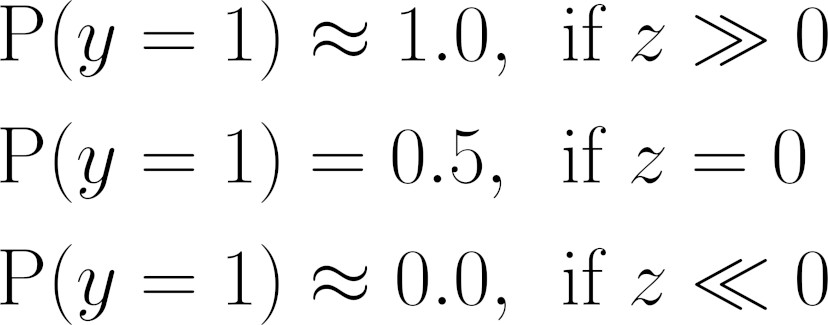
For really large positive and negative logit values (z), we would like to have:

Probabilities assigned to different logit values (z)

We still need to figure out a function that maps logit values into probabilities. We’ll get there soon enough, but first, we need to talk about…

Odds Ratio

What are the odds?!

This is a colloquial expression meaning something very unlikely has happened. But odds do not have to refer to an unlikely event or a slim chance. The odds of getting heads in a (fair) coin flip are 1 to 1 since there is a 50% chance of success and a 50% chance of failure.

Let’s imagine we are betting on the winner of the World Cup final. There are two countries: A and B. Country A is the favorite: It has a 75% chance of winning. So, Country B has only a 25% chance of winning. If you bet on Country A, your chances of winning—that is, your odds (in favor)—are 3 to 1 (75 to 25). If you decide to test your luck and bet on Country B, your chances of winning—that is, your odds (in favor)—are 1 to 3 (25 to 75), or 0.33 to 1.

The odds ratio is given by the ratio between the probability of success (p) and the

probability of failure (q):

Odds ratio

In code, our odds_ratio() function looks like this:

def odds_ratio(prob):

return prob / (1 - prob)

p = .75

q = 1 - p

odds_ratio(p), odds_ratio(q)

*Output*

(3.0, 0.3333333333333333)

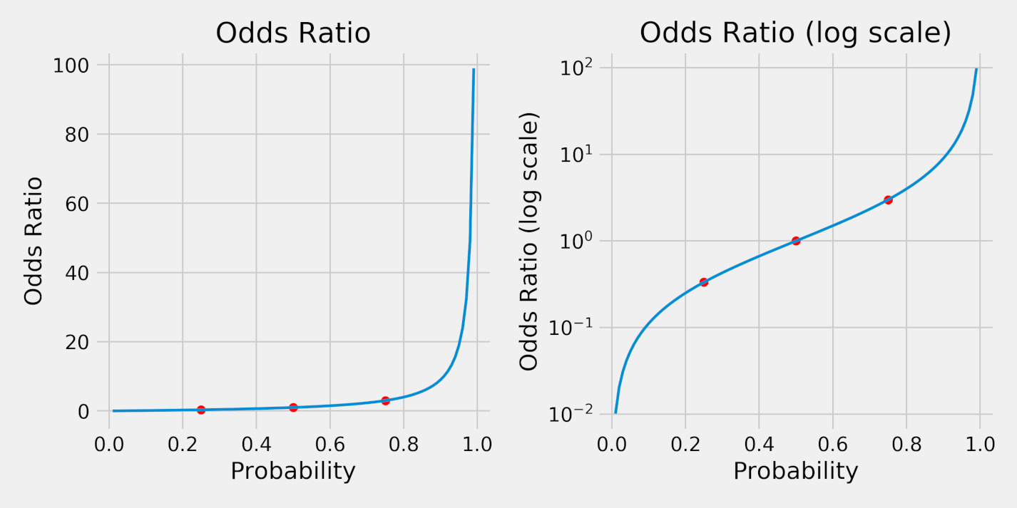
We can also plot the resulting odds ratios for probabilities ranging from 1% to 99%. The red dots correspond to the probabilities of 25% (q), 50%, and 75% (p).

Odds ratio

Clearly, the odds ratios (left plot) are not symmetrical. But, in a log scale (right plot), they are. This serves us very well since we’re looking for a symmetrical function that maps logit values into probabilities.

Why does it need to be symmetrical?

If the function weren’t symmetrical, different choices for the positive class would produce models that were not equivalent. But, using a symmetrical function, we could train two equivalent models using the same dataset, just flipping the classes:

• Blue Model (the positive class (y=1) corresponds to blue points)
  • Data Point #1: P(y=1) = P(blue) = .83 (which is the same as P(red) = .17)
• Red Model (the positive class (y=1) corresponds to red points)
  • Data Point #1: P(y=1) = P(red) = .17 (which is the same as P(blue) = .83)

##Log Odds Ratio

By taking the logarithm of the odds ratio, the function is not only symmetrical, but also maps probabilities into real numbers, instead of only the positive ones:

Log odds ratio

In code, our log_odds_ratio() function looks like this:

def log_odds_ratio(prob):

return np.log(odds\_ratio(prob))

$$p = .75$$

$$q = 1 - p$$

$$\log_odds_ratio(p), log_odds_ratio(q)$$


*Output*

(1.0986122886681098, -1.0986122886681098)

As expected, probabilities that add up to 100% (like 75% and 25%) correspond to

log odds ratios that are the same in absolute value. Let’s plot it:

Log odds ratio and probability

On the left, each probability maps into a log odds ratio. The red dots correspond to probabilities of 25%, 50%, and 75%, the same as before.

If we flip the horizontal and vertical axes (right plot), we are inverting the function, thus mapping each log odds ratio into a probability. That’s the function we were looking for!

Does its shape look familiar? Wait for it…

From Logits to Probabilities

In the previous section, we were trying to map logit values into probabilities, and we’ve just found out, graphically, a function that maps log odds ratios into probabilities.

Clearly, our logits are log odds ratios :-) Sure, drawing conclusions like this is not very scientific, but the purpose of this exercise is to illustrate how the results of a regression, represented by the logits (z), get to be mapped into probabilities.

So, here’s what we arrived at:

Equation - Regression, logits, and log odds ratios

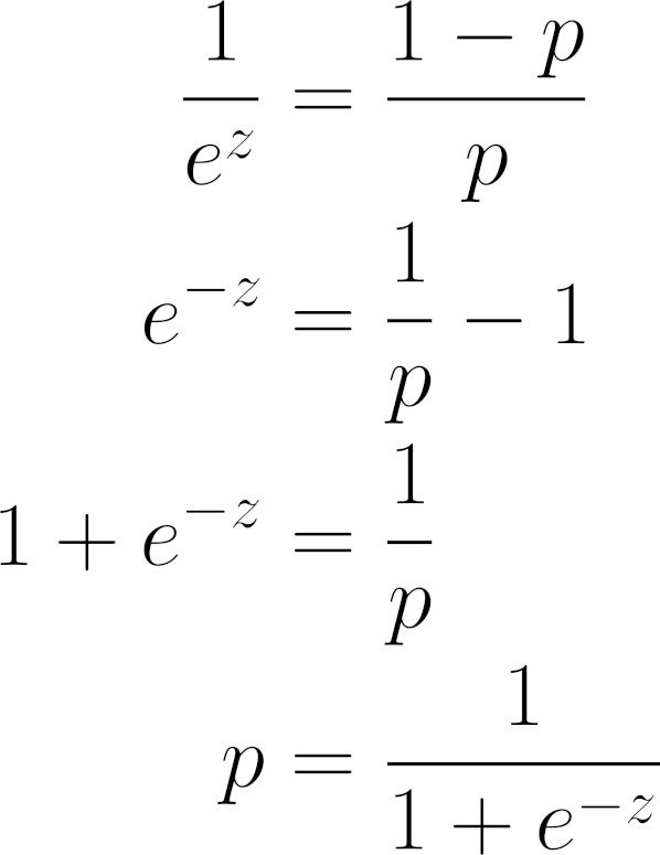
Let’s work this equation out a bit, inverting, rearranging, and simplifying some terms to isolate p:

Equation - From logits (z) to probabilities (p)

Does it look familiar? That’s a sigmoid function! It is the inverse of the log odds ratio.

Equation - Sigmoid function