An API for The National Hockey League (NHL)
Table of contents
- Experiment Tracking
- Feature Engineering I
- Baseline Models
- Feature Engineering II
- Advanced Models
- Give Best Shot
- Evaluate on Test Set
- Conclusion
Experiment Tracking
All the following experiments were carefully tracked using Comet ML. This is an important step that we took to make our experiments reproducible.
Feature Engineering I
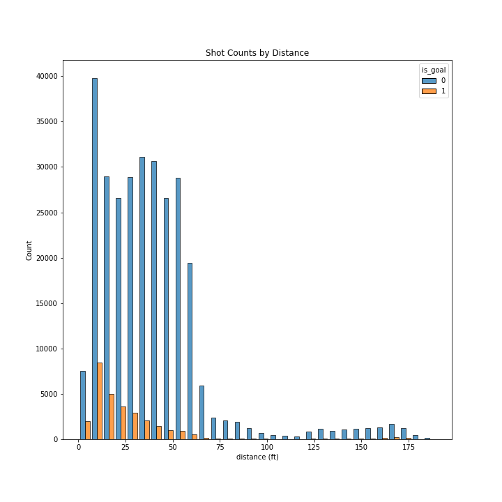
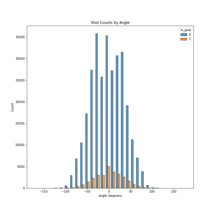
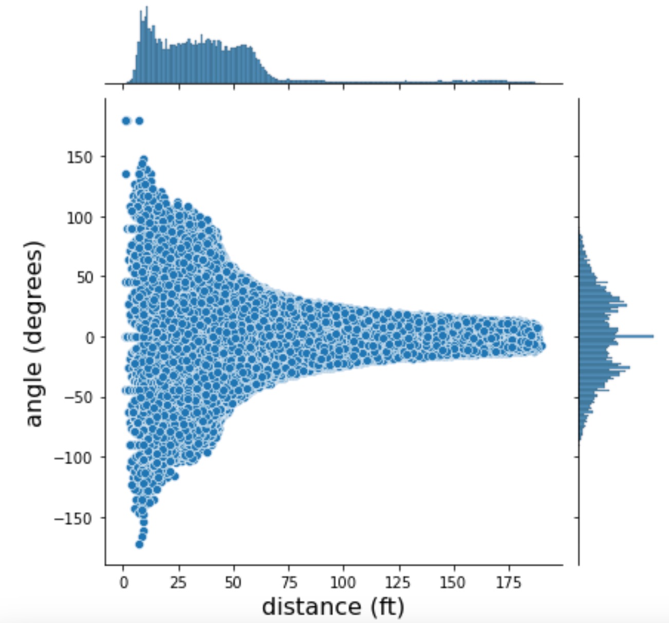
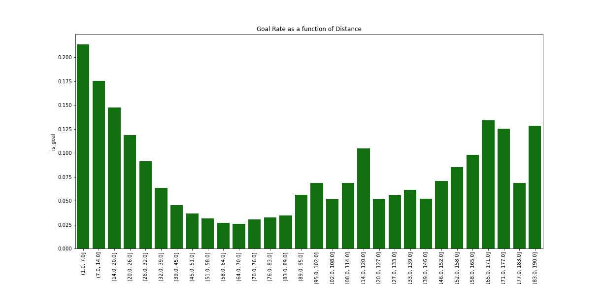
Goal rate as a function of distance
First, there is a relationship between the distance and the probability of a goal, such as the probability of a goal is inversely proportional to distance when the distance is less than approximately 60 ft.
Second, there is some (stochastic) probability of a goal with shots taken at approximately more than 60 feet which can be in some cases higher than for goals taken at about 60 feet.
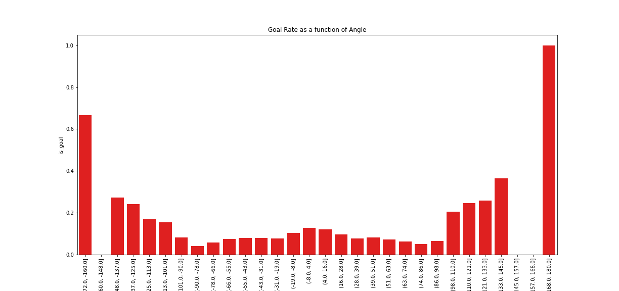
Goal Rate as a function of Angle
First, there is slightly more chance that a goal results in a goal when it is taken from in front of the goal, but only when the shot is taken at less than 90 degrees.
Second, even though shots taken from in front of the goal (i.e. at an angle close to zero) are the most common, these are not the most successful in achieving a goal. The likelihood of a goal increases as a proportion to the angle, specifically when the angle is greater than approximately 90 degrees.
Third and very importantly, the distribution is symmetric only in its middle part. There is a very clear asymmetry when comparing the extremities of the distribution. Specifically, shots taken at very high angles (approximately more than 150 degrees) are more likely to achieve a goal when taken from the side which corresponds to the right-hand side of the goalie. We need to bear in mind that most goalies are right-handed and hold their hockey sticks on the left side as all other players, and therefore their right side is relatively unprotected. This might explain why shots taken from the far-right-hand side of the goalie are much more likely to result in a goal.
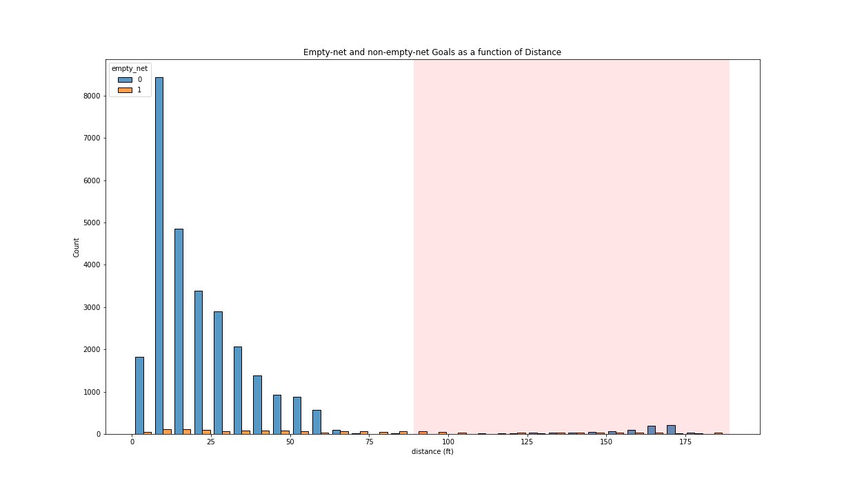
The distribution is coherent with domain-specific knowledge (i.e. that “it is incredibly rare to score a non-empty net goal on the opposing team from within your defensive zone”). Indeed, a few successful goals (in total, 795 goals for the complete seasons involved) were shot from more than 89 feet. Based on this, it seems that the features are correct, and we cannot find any events that have incorrect features.
Note: Here, we indicate the approximate defense zone by a red shade, from 89 feet from the goal up to 180 feet. This is an approximation because the distance is measured from the goal and thus is not always calculated perpendicular to the central line.
Baseline Models
Links to Various Logistic Models on Comet ML platform.
- Logistic model trained on angle
- logistic model trained on distance
- logistic model trained on distance and angle
The accuracy is 90% correctly predicted as compared total. However, accuracy is not the right metric to use in this setting because there is a high imbalance between goals and missed shots, in the order of 1:10. Indeed, we can see that from the classification report its clear that all the test data (validation data) has been predicted to be 0s (missed shots) as the output. Therefore, even though this model achieved 90% accuracy, it was not successful in predicting any goal. This is why accuracy is not the correct metric, and other metrics like ROC AUC should be used.
The model based on both distance and angle (distance_angle) and that based on distance alone (distance) are the two best models when considering the ROC AUC. Indeed, their area under the curve is the largest one (0.67964). In comparison, the two other models (random_base_line and the angle ones) are not distinguishable from random results, i.e. their ROC curve follows closely the bisector line.
As expected, the highest percentiles observations (the observations that have the highest predicted probability of being a goal) have the highest proportion of goals; however only for the distance_angle and distance_models. More specifically, the proportion of goals raises to approximately 20% for the highest-percentile observations, while it gets close to 5% for the lowest-percentile observations. For the other two models, the proportion of goals is the same in all percentiles and is close to 10% which is the overall proportion of goals in any random sample from the dataset.
There is a non-linear relationship between the model probability percentile and the cumulative proportion of goals, but only for the distance and distance_angle curves. Specifically, for these two curves, the more the model probability percentile increases, the more the proportion increases, but the slope decreases. In comparison, the two other curves, show a close-to-linear relationship.
This difference in slope between models reflects the same finding as the previous graph, i.e. the highest percentiles observations have the highest proportion of goals only for the distance_angle and distance_models. In other words, these two models were successful in learning to predict goals.
From the Calibration plot, we see that fraction of positive cases is always the same whatever the mean predicted probability is, for every four models tested. In all cases, the fraction of positive cases is equal to 1:10 which is the (approximate) overall ratio of goals as compared to all shots in the complete sample.
This could induce us to think that all four models performed the same and that none of these models succeeded in predicting goals from the data. However, we need to take note that the calibration plot - like the accuracy metric - is not the most adequate way to evaluate a model when the predicted event is rare (in our case, 1:10). From the previous plots, we showed that the distance_angle and distance models show some success in predicting goals, which is not apparent from the calibration plot. This observation highlights the importance of choosing the correct metric and correct plots when evaluating a model.
Feature Engineering II
Here is a list and description of all features that we engineered:
• distance: distance (feet) between the event and the center of the net at which the shot is aimed.
• angle: angle (degrees) between the center line and the event. One can imagine this angle by putting himself in the position of the goalie: if the shot is taken from right in front, the angle is equal to zero.
• empty_net: shot was taken against a net without a goalie.
• game_period: period number during the game.
• distance_from_last_event: distance (feet) between the last event and the present event.
• rebound: whether this shot follows another shot.
•change_in_shot_angle: difference (degrees) in angle between the present shot and the previous event, if this event was also a shot.
• speed: average speed (feet by second) of the puck between the last and the present shot.
•x_coordinate: coordinate (feet) taken from the center of the ice.
•y_coordinate: coordinate (feet) taken from the center of the ice.
•game_seconds: time (seconds) as measured from the beginning of the game.
•shot_type: type of shot, one-hot encoded into 8 indicator variables, i.e. Backhand, Deflected, Slap Shot, Snap Shot, Tip-In, Wrap-around, Wrist Shot, and NA.
•last_event_type: type of the last event, one-hot encoded into 9 indicator variables, i.e. Blocket shot, Faceoff, Giveaway, Goal, Hit, Missed shot, Penalty, Shot, Takeaway.
Link to the filtered data frame
Advanced Models
Best XGBoost Model
Hyperparameter Tuning and Model Comparison
In each experiment, we try to find the best possible values of hyperparameters utilizing a grid search. We split the train set into stratified 3-fold cross-validation and take mean performance to decide the best performing set of hyperparameters. As explained before, we have a class imbalance in our data, which is better captured by the F1 Score metric.
To compare models based on their performance, we used the same train-validation split for all models. This guarantees that the performance metrics are obtained on the same dataset, therefore we can compare the model’s performance. Specifically train-validation split was an 80%-20% split obtained with random splitting, and we used the same for all models.
Handling Class Imbalance
We tried 2 methods to handle the huge class imbalance present in the data:
- Class weighting the objective function:
In this method, due to the nature of the algorithm, we employ gradient updates for parameter optimization. While aggregating the gradients over the samples, we apply weights to them based on the number of occurrences in training sets. We scale the gradients for the majority and minority classes to achieve balance.
- ADASYN algorithm:
In this method, we oversample the minority class so that we have enough samples to learn from. The new samples are generated synthetically.
We compare the results from both this method for all 3 XGBoost configurations and found that we don’t find much difference in performance metrics(F1 Score). The results reported are from utilizing class weighting.
XGBoost classifier trains on distance and angle
First, we create XGBoost baseline to compare the logistic baseline, with just ‘distance’ and ‘angle’ as the features. To tackle the class imbalance problem, the Following are the hyper-parameters for grid search:
{"learning_rate": [0.1, 0.3], "max_depth": [2, 4, 6], "n_estimators": [4, 6, 8, 10], "objective": ["binary:logistic"], "reg_alpha": [0.1, 1.0]}
We get the following hyper-parameters for the best estimator:
{'learning_rate': 0.3, 'max_depth': 6, 'n_estimators': 6, 'objective': 'binary:logistic', 'reg_alpha': 1.0}
Here, we compare the performance of XGBoost based on features distance and angle, to that of a simple logistic regression trained using the same features. The ROC AUC=0.66892 obtained for the logistic regression was, while that obtained with XGBoost is ROC AUC= 0.708. We consider that there is no significant difference here between the performance of these two models. This is likely explained by the fact that they were trained on only two features, therefore the XGBoost does not have much advantage over the logistic model here.
XGBoost classifier trains on all features
Next, we use all the features as defined in the section feature engineering 2. We use the same configuration of training/validation split and grid search with cross-validation as the XGBoost baseline. As explained above, the F1 Score is used as a metric for selecting the best performing model. Following are the hyperparameters for hyperparameter tuning:
{"learning_rate": [0.3], "max_depth": [4, 6, 8], "n_estimators": [25, 45, 70, 100], "objective": ["binary:logistic"], "reg_alpha": [1.0], "reg_lambda": [1.0]}
We get the following configuration for the best estimator:
{'learning_rate': 0.3, 'max_depth': 4, 'n_estimators': 45, 'objective': 'binary:logistic', 'reg_alpha': 1.0, 'reg_lambda': 1.0}
Performance of the model
We notice a small improvement in the performance of the model when using all features (ROC AUC = 0.757) as compared to using only distance and angle (ROC AUC = 0.708).
Feature Selection
We used a range of methods of feature selection that cover all types: filter, wrapper, and embedded methods. Here, we discuss and compare the results of each method. For each method, we keep the 5 highest-scoring features; and at the end, we will compute the intersection and union between all sets of obtained features.
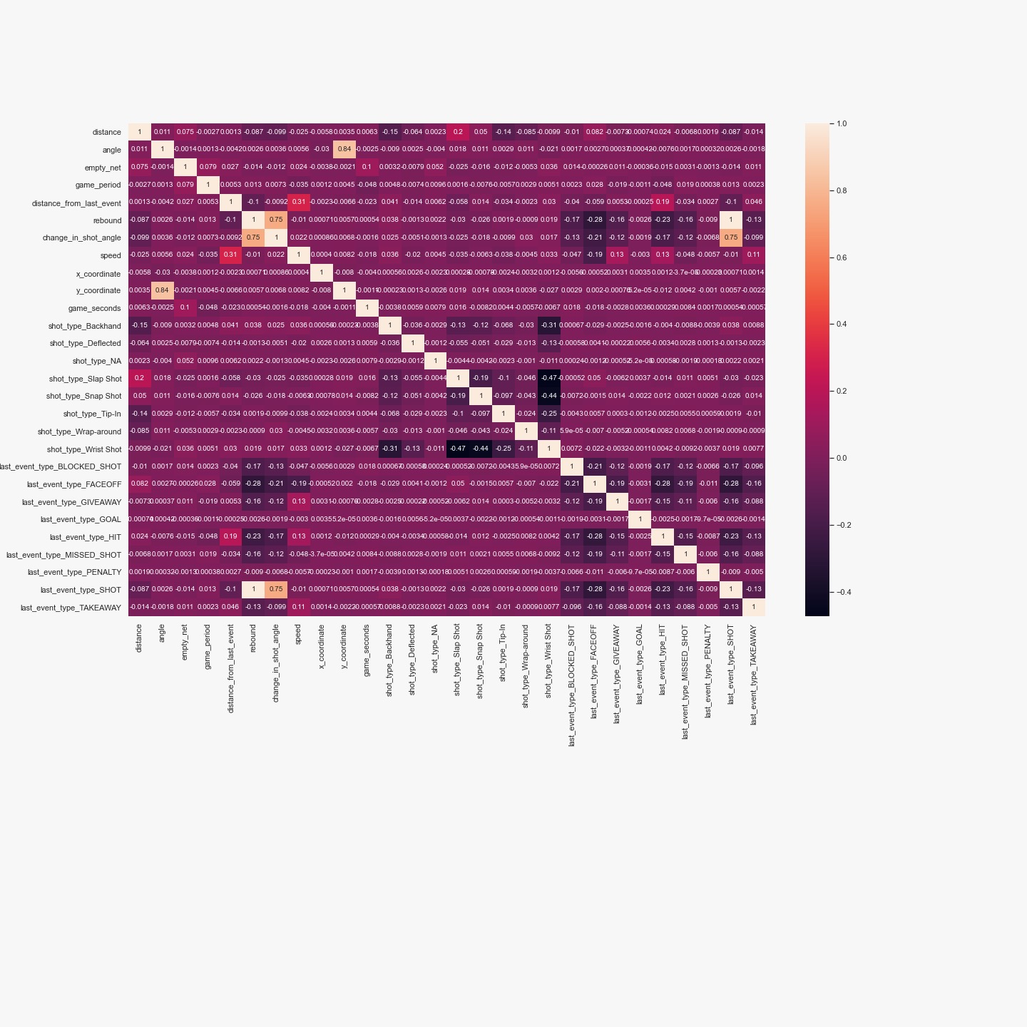
Before starting feature selection, we notice that some features are correlated. Specifically, the angle is correlated with y_coordinate (r=0.84) and change_in_shot_angle, as well as rebound, are correlated with last_event_type_SHOT (because these variables were defined based on one another). This means that there is probably some redundant information in these variables that needs to be parsed using feature selection.
Filter Methods
We first used a variance threshold of 80%, thus removing all features that are either one or zero in more than 80% of the sample.
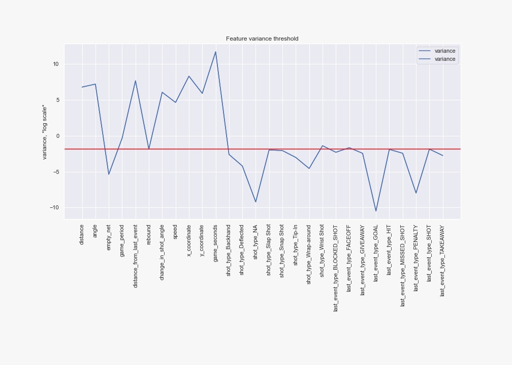
Then, we decided to keep only the 5 features with the highest variance, to stay coherent with the general method for all feature selection methods. The 5 top-ranked features were: ['distance', 'angle', 'distance_from_last_event', 'x_coordinate', 'game_seconds']
Then, we also used univariate feature selection while using 6 different criteria. That is, we used all the methods available in scikit-learn that can be used for a classification task and that accept both positive and negative inputs:
• ANOVA F-value between label/feature for classification tasks.
• Mutual information for a discrete target.
• Percentile of the highest scores.
• False positive rate test.
• Estimated false discovery rate.
• Family-wise error rate.
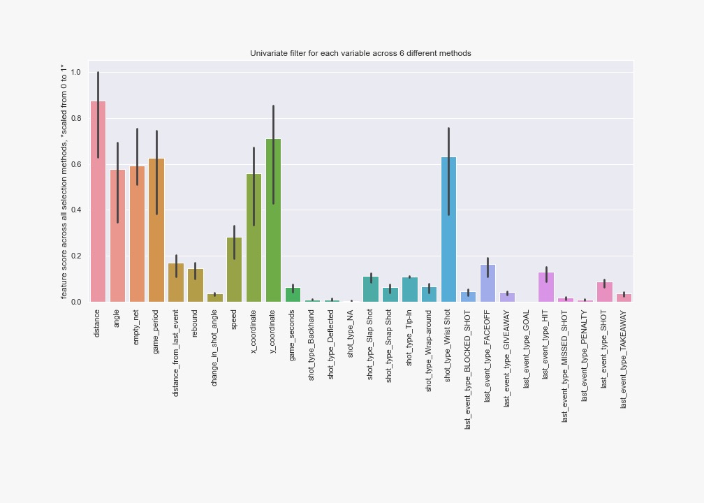
The 5 top-ranked features (on average among methods) were: ['distance', 'empty_net', 'game_period', 'y_coordinate', 'shot_type_Wrist Shot']
Wrapper methods
We used both forward search and backward search using logistic regression, setting the number of features to select equal to 5. For these methods, we scaled all features because this was needed for the logistic regression to converge.
Forward search resulted in these features:
['distance', 'angle', 'empty_net', 'game_period', 'distance_from_last_event']
Backward search: the model does not converge.
Embedded methods
We evaluated the coefficients from l2-penalized logistic regression, as well as that of Linear Support Vector Classification. Note that we are interested in the magnitude, therefore in the absolute value of the coefficient. For these methods, we scaled all features because this was needed for the logistic regression to converge.
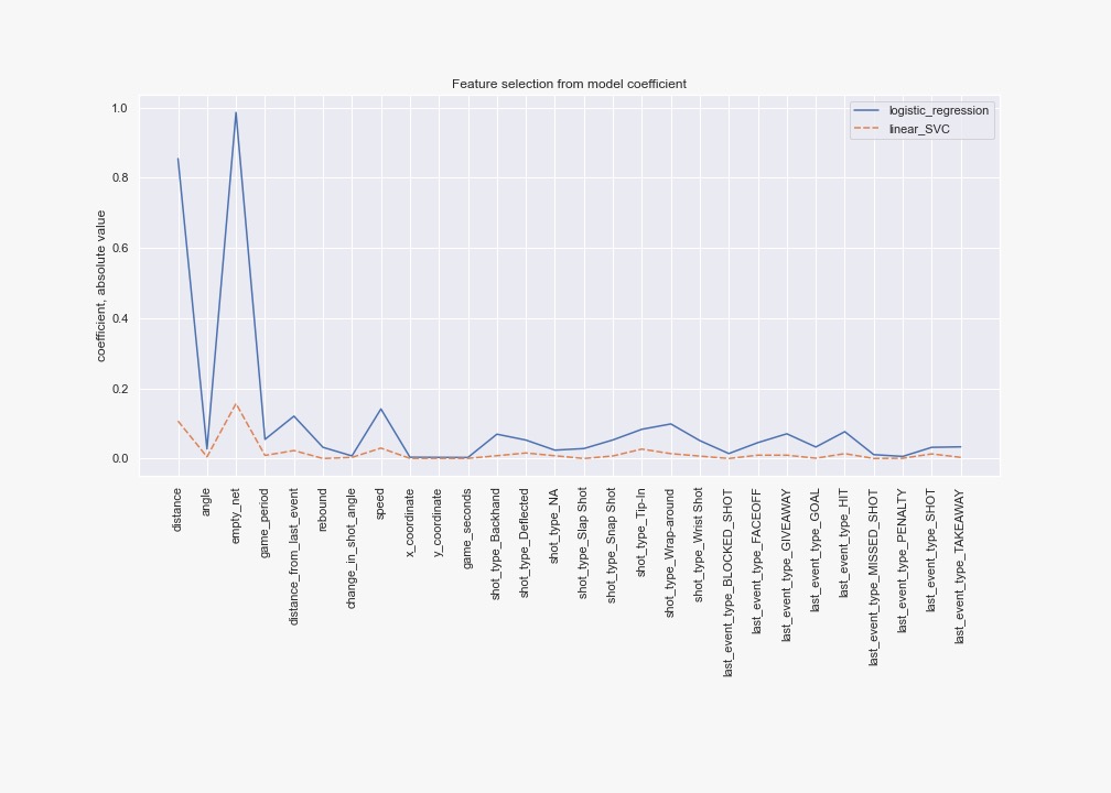
For logistic regression, the 5 top-ranked features were: [distance, empty_net, distance_from_last_event, speed, shot_type_Wrap-around]
For linear SVC, the 5 top-ranked features were: [distance, empty_net, distance_from_last_event, speed, shot_type_Tip-In]
SHAP Features
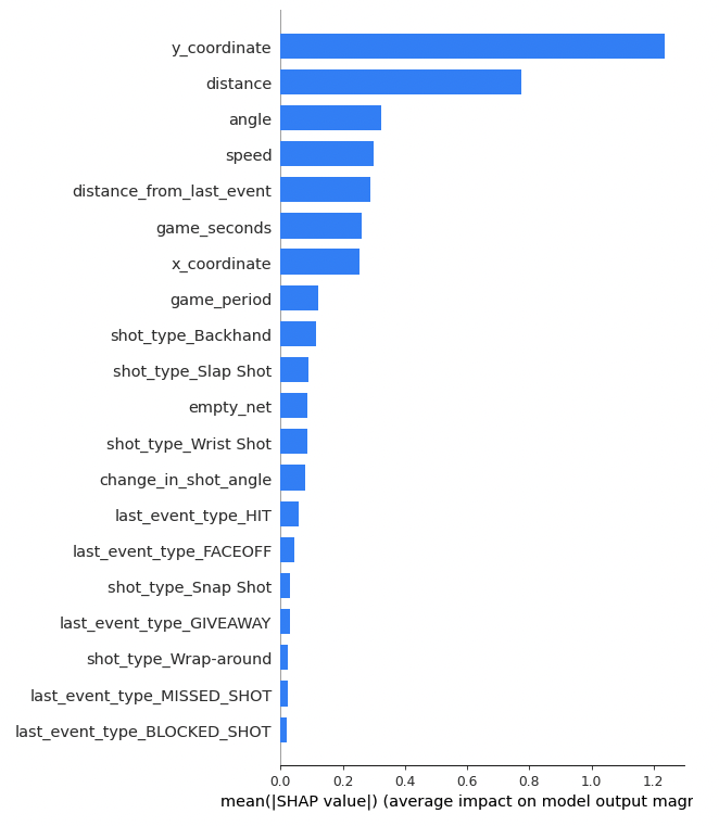
We also use SHAP algorithm’s tree explainer which operates on adding a particular feature to a subset of features and assigns importance based on its contribution. We use all features XGBoost model to generate the Shapley values and in turn, get the feature importance. The following plot describes this:
Summary and consensus among feature selection methods
In summary, we used 2 filters (including 6 different univariate methods) plus wrapper two more embedded and SHAP for a total of six different methods. From these, we compute the intersection and union of sets of 5 top-ranked features from each method. We obtain:
Intersection: [distance]
Union: [angle, distance_from_last_event, empty_net, shot_type_Wrap-around, y_coordinate, speed, distance, x_coordinate, game_period, shot_type_Tip-In, shot_type_Wrist Shot, game_seconds]
XGBoost train on selected features
We utilize the following hyper-parameter configuration for grid search:
{"learning_rate": [0.1, 0.4], "max_depth": [4, 6, 8], "n_estimators": [25, 35, 50, 70, 100], "objective": ["binary:logistic"], "reg_alpha": [1.0], "reg_lambda": [1.0]}
Performance of the model It is important to notice that the feature selection is achieved in improving the model performance. While the model with all features had a ROC AUC = 0.708, the model with fewer but rigorously selected features had a ROC AUC = 0.75. This reflects the fact that sometimes adding more features mostly adds more noise. This is an illustration of why feature selection is important.
Give Best Shot
We trained and evaluated a variety of different models. Considering that our dataset was unbalanced (goals represent 1/10 events), models were trained such as to obtain the best performance as measured by ROC-AUC.
- K-nearest-neighbours
- Random Forests
- Decision trees
- Neural Networks - which resulted in our Best Model
We also used a variety of other approaches including stratified train-test split and k-fold cross-validation.
At this point, we also went back to the feature selection section, and we improved the variety of our feature selection algorithm. We improved the general pipeline of our feature selection (see the relevant section) such as to include a variety of filter, embedded and wrapper methods, to achieve a consensus among these methods. We noted that different feature selection methods resulted in different sets of features, and we reasoned that these sets might have importance for different reasons. We thus used the union of all sets as the final set of features, to include all relevant information. Models were thus trained with the final set of features.
# k-nearest-neighbours We trained a kNN using Scikit-learn. We used Euclidean distance as a distance metric. We searched for the best hyperparameter i.e., the one that maximized the area under the ROC curve (ROC AUC), by iteratively training KNN while using different values of k = 1, 2, 3, …, 50.
kNN resulted in high accuracy and a satisfying ROC AUC (AUC=0.71)). However, when we evaluated the confusion matrix, we noticed that there were very few events predicted to be goals: the model predicted most events to be missed shots, and therefore is not an adequate model for this data and setting where we aim to predict goals. We explain this observation by the imbalance of our dataset, in which Euclidean distance could not establish a space where a majority of points would be goals: in nearly all cases, the majority of points would still be missed shots, and therefore kNN nearly always predicted shots to be missed shots.
Random Forests
We trained a Random Forest model using Scikit-learn. After some trials, we finally used the following hyperparameters: number of trees as 1,000 and Gini impurity as the criterium for the split.
We got a ROC AUC = 0.72. However, like the kNN, when we evaluated the confusion matrix, we noticed that there were very few events predicted to be goals: the model predicted most events to be missed shots, and therefore is not an adequate model for this data and setting where we aim to predict goals.
Decision Trees
We trained a Decision Tree model using Scikit-learn. We selected hyperparameters using a randomized search.
This model performed the worst among those tested here, as we got a ROC AUC = 0.65.
Neural Networks are our Best Model
Link of the model in Comet ML platform.
We trained Neural Networks using PyTorch. After exploring a variety of loss functions and optimizers, we finally selected AdamW as an optimizer, and Cross Entropy as a loss function because it optimized model performance. The model was then trained iteratively using the settings available in PyTorch. Importantly, the main turnaround for increasing accuracy was introducing class weights in my loss function which will penalize more on the class which has a low no of data points hence giving more importance.
The Neural Networks obtained the best ROC-AUC ex-aequo with the Random Forest (i.e. we consider AUC=0.72 to be not significantly different from that of Random Forest). However, we consider the Neural Networks to be our best model because the examination of the confusion matrix reveals a much better classification than for Random Forest.
Evaluate on Test Set
Regular season:
For the Regular Season, the model’s performed similarly in the final evaluation set as they did in the training set. The best model based on ROC-AUC was again the Neural Networks. All curves as well as ROC-AUC metrics are close to those observed during training for the same models. This confirms that our models were not over-fitted during training, as there don’t seem to be issues such as leakage or improper splitting that could have resulted in over-fitting.
Playoffs:
For the Playoffs, there was a very interesting discrepancy between model performance in the training set and that observed here in the final evaluation set. Specifically, performance is lower in the final evaluation set than in the training test and for all models. This is likely explained by the fact that most observations in the training set were from the Regular Season: Playoffs represent only 6.4% (20280/315725) of all observations. Goals made during Playoffs are likely predicted by different parameters than those made during Regular Season, because of the context and rules. Therefore, the models were trained mostly to predict goals during the Regular Season and thus performed poorly when evaluated only during the Playoff season. Possible solutions to this problem would be to train specific models only for the Playoff season, or to better account for the effect of the season on how the season affects the predictive power of other variables.
Finally, we note that in this case, XGBoost performs better than other models, with a ROC-AUC=0.61. This might be explained by the specificity of this model, i.e. its ensemble methodology and its ability to learn multiple weak models to build a strong robust model which is flexible in many scenarios.
Conclusion
The present project is a good example of how sports data can be obtained from a publicly available API and made into a data format that can be used for advanced, interactive visualizations, as well as a variety of Machine Learning models.
This project involved predicted a relatively rare (10%) event - goals. It illustrates how feature engineering, feature selection, and finally hyperparameter tuning and model selection can achieve a good model generalizability to the evaluation set. The fact that the generalizability was poor to the part of the evaluation set that represented the playoffs illustrates how it is important for the training set to be representative of the evaluation set in all aspects. This also illustrates how some models might have better generalizability in such a context (i.e. XGBoost).
Some limitations of the present project involve the fact that we used a simple train-test split. The method that we used therefore did not permit us to assign a confidence interval to the performance metrics, such as to compare whether the performance of the models was significantly different from one another.