Deep Learning with PyTorch Step-by-Step

Optimizer for NN:

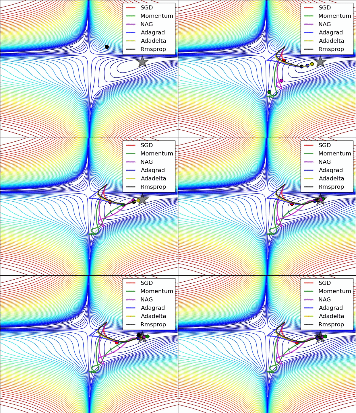
What if we had a whole lot of parameters using the computed gradients? We need to use one of PyTorch’s optimizers, like SGD, RMSprop, or Adam. There are many optimizers: SGD is the most basic of them, and Adam is one of the most popular. Different optimizers use different mechanics for updating the parameters, but they all achieve the same goal through, literally, different paths.The following animation shows a loss surface,the paths traversed by some optimizers to achieve the minimum (represented by a star).

Remember, the choice of mini-batch size influences the path of gradient descent, and so does the choice of an optimizer.

Most modern neural networks are trained using maximum likelihood. This means that the cost function is simply the negative log-likelihood, equivalently described as the cross-entropy between the training data and the model distribution. This cost function is given by \(J(θ) = \log p_{model}(y | x)\) The specific form of the cost function changes from model to model, depending on the specific form of \(\log p_{model}\) The expansion of the above equation typically yields some terms that do not depend on the model parameters and may be discarded. For example, if \(p_{model}(y | x) = N(y; f(x; θ), I)\),then we recover the mean squared error cost, \(J(θ) = 1\)

In this blog, we will:

• define a simple linear regression model

• walk through every step of gradient descent: initializing parameters, performing a forward pass, computing errors and loss, computing gradients, and updating parameters

• understand gradients using equations, code, and geometry

• understand the difference between batch, mini-batch, and stochastic gradient descent

• visualize the effects on the loss of using different learning rates

• understand the importance of standardizing / scaling features